Q1 Stability vs Volatility
Use the level switcher to focus on city or cinema performance. Each view keeps charts and spotlights in sync.
Question focus
Identify cities and cinemas with steady weekly revenue versus highly volatile ones, using risk-adjusted performance to separate safe bets from high-upside risks.
City level
City view shows which locations are stable versus volatile.
Stability vs volatility map
Average weekly gross vs volatility (CV). Bigger bubbles = larger markets.
Revenue share vs location share
Compare each risk category's share of revenue vs its share of cities.
City spotlights
Top stable and volatile cities by total gross.
| Type | Location | Total gross | CV |
|---|---|---|---|
| Stable | Victoria (inc TAS) | West Melbourne | $473,075,918 | 0.60 |
| Stable | New South Wales (inc ACT) | West and Blue Mountains | $312,742,841 | 0.60 |
| Stable | Victoria (inc TAS) | South East Melbourne | $295,602,124 | 0.72 |
| Stable | New South Wales (inc ACT) | Parramatta & Ryde | $232,923,669 | 0.72 |
| Stable | Queensland | Brisbane - South | $168,627,300 | 0.66 |
| Stable | Victoria (inc TAS) | North East Melbourne | $100,542,920 | 0.61 |
| Volatile | New South Wales (inc ACT) | Sutherland & St George | $27,948,256 | 1.63 |
| Volatile | New South Wales (inc ACT) | Illawarra | $11,298,562 | 1.14 |
| Volatile | New South Wales (inc ACT) | City and Inner South | $10,451,936 | 2.17 |
| Volatile | Queensland | Townsville Region | $8,728,658 | 1.34 |
| Volatile | Victoria (inc TAS) | Shepparton | $7,684,032 | 1.13 |
| Volatile | Victoria (inc TAS) | Ballarat | $7,543,310 | 1.11 |
Analyst Appendix
Action takeaway
Start releases in safer, high risk-adjusted locations to secure baseline revenue, then test a limited set of higher-risk markets with tighter monitoring and flexible screen holds.
CV distribution by risk category
Shows the spread of volatility within each risk tier.
Revenue-weighted CV histogram
Highlights where most revenue sits across volatility levels.
Insight: In this chart, most revenue comes from lower-volatility cities (around CV ~0.6-0.9), while highly volatile cities contribute much less total revenue.
Volatility heatmap by week
Relative weekly performance for top stable and volatile cities.
Q2 Early Adopter vs Slow Burn
Use the level switcher to focus on state, city, or cinema performance. Each view includes timing maps, revenue distribution, speed charts, and highlights.
Question focus
Determine where revenue arrives fast (weeks 1-2) versus slowly, and classify each state, city, and cinema as early adopter, balanced, or slow-burn.
Action takeaway
Front-load marketing and screens in early-adopter locations for quick payback, then extend runs and steady spend in slow-burn markets to capture long-tail revenue.
State level
State view shows national early-adopter patterns and slow-burn regions.
Timing map
Early share vs total gross with timing thresholds.
Revenue distribution
Total gross spread by timing type.
Ramp-up speed
Median and IQR weeks to reach 80% of total gross.
Revenue share vs location share
Compare revenue share against share of locations in each timing type.
State spotlights
Top early adopters and slow-burn states.
| Type | Location | Total gross | Early share |
|---|---|---|---|
| Early adopter | Northern Territory | $25,038,997 | 0.95 |
| Early adopter | Queensland | $357,845,979 | 0.95 |
| Early adopter | Western Australia | $290,639,729 | 0.93 |
| Early adopter | South Australia | $231,682,571 | 0.92 |
| Early adopter | Victoria (inc TAS) | $1,217,784,910 | 0.90 |
| Slow burn | New South Wales (inc ACT) | $996,715,591 | 0.90 |
| Slow burn | Victoria (inc TAS) | $1,217,784,910 | 0.90 |
| Slow burn | South Australia | $231,682,571 | 0.92 |
| Slow burn | Western Australia | $290,639,729 | 0.93 |
| Slow burn | Queensland | $357,845,979 | 0.95 |
Analyst Appendix
Timing class mix by state
Stacked view of timing classes across states.
Cumulative revenue share by week
Small multiples by timing class show ramp-up patterns.
Pareto by timing class
How concentrated revenue is within each timing class.
Q3 Seasonality Story
Use the level switcher to focus on state, city, or cinema seasonality. Each view keeps charts and spotlights in sync.
Question focus
Map peak and quiet ISO weeks by state, city, and cinema, and relate demand to competition to find strong and weak release windows.
Action takeaway
Schedule tentpoles in peak weeks and top-performing locations, use high-demand/low-competition windows for mid-tier titles, and reduce spend during troughs.
State level
National timing view. Use this to spot weeks that peak across multiple states.
Weekly seasonality map
Seasonality index above 1 means above-median demand for that state.
Seasonality distribution by state
Violin width shows how volatile each state is across the year.
Top states timing profile
Largest markets by total gross with a median benchmark.
National peaks and troughs by week
Average seasonality index across states by ISO week.
Peak and quiet weeks (national average)
Top and bottom weeks based on average seasonality index.
| Type | Week | Seasonality Index |
|---|---|---|
| Peak | W33 | 3.84 |
| Peak | W13 | 3.23 |
| Peak | W18 | 2.65 |
| Peak | W31 | 2.56 |
| Quiet | W46 | 0.00 |
| Quiet | W01 | 0.15 |
| Quiet | W21 | 0.28 |
| Quiet | W10 | 0.29 |
Q4 Catchment Model
Q1–Q3 describe where Indian films sell. This section asks why, regressing weekly cinema gross on SA4 catchment demographics.
Question focus
Explain the spatial pattern with structural demand: Indian-ancestry share, density, income, age, and local competition, controlling for the film and the calendar week.
Headline result
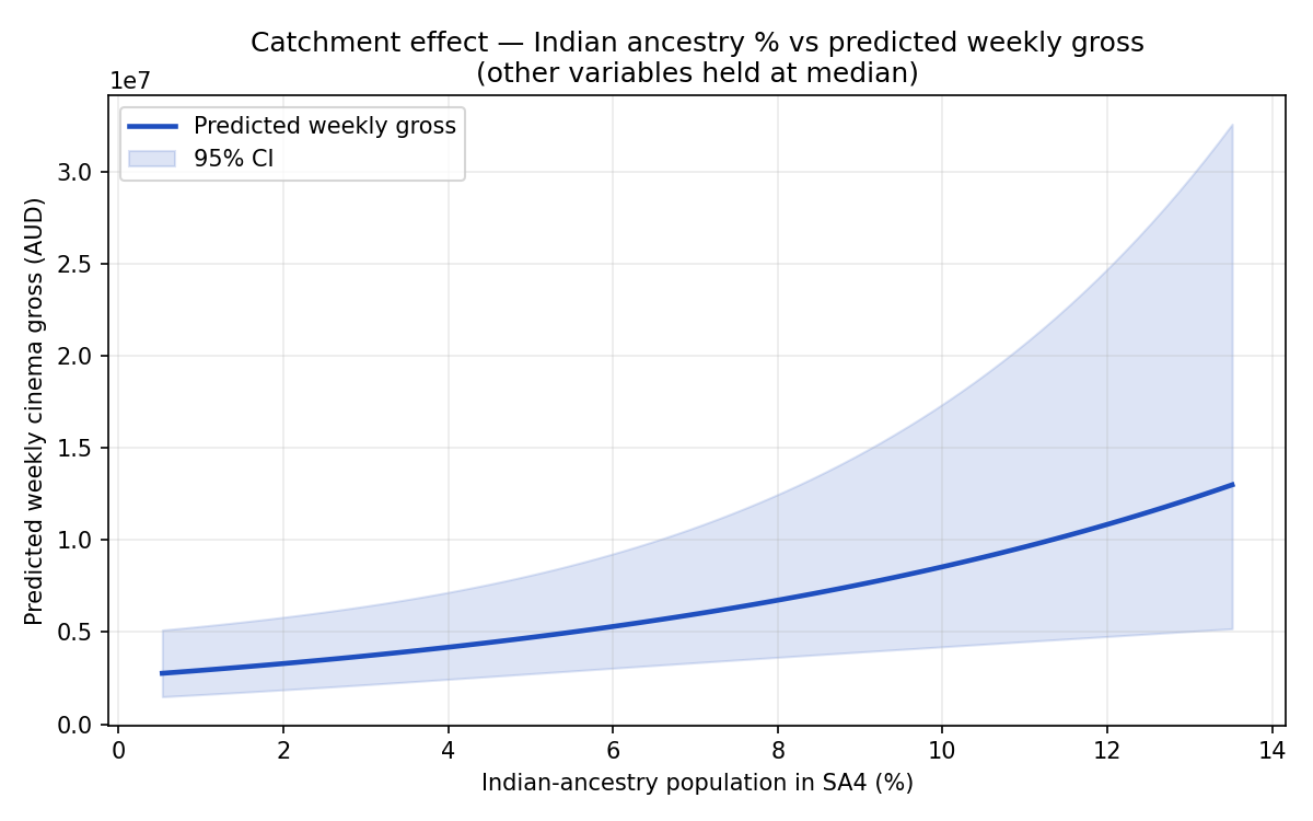
Holding the film, the calendar week, income, and age structure constant, a +5 percentage-point increase in the Indian-ancestry share of a cinema's SA4 catchment is associated with a +81.6% change in weekly gross (95% CI: +21.4% to +171.5%; n = 10,498; R² = 0.42 in full-FE spec).
This is the structural demand signal that Q1's "Safer / Volatile" labels were picking up indirectly. Cities flagged as "Safer" tend to sit on SA4s with a thick Indian-Australian population, and the stability is a fundamentals story, not statistical luck.
Coefficients across nested specifications
| Variable | M1 | M2 | M3 |
|---|---|---|---|
| pct_indian_ancestry | 0.095*** [0.043, 0.147] | 0.100*** [0.029, 0.171] | 0.119*** [0.039, 0.200] |
| log_pop_density | 0.099*** [0.025, 0.173] | 0.112** [0.026, 0.198] | 0.122*** [0.031, 0.214] |
| nearest_competitor_km | 0.000 [-0.001, 0.001] | 0.000 [-0.001, 0.002] | 0.000 [-0.002, 0.002] |
| median_income_k | n/a | -0.209 [-0.638, 0.220] | -0.188 [-0.652, 0.275] |
| median_age | n/a | -0.021 [-0.074, 0.032] | -0.021 [-0.078, 0.036] |
| N | 10,498 | 10,498 | 10,498 |
| R² | 0.070 | 0.155 | 0.423 |
Coefficients on log(gross). Standard errors clustered on cinema. *** p<0.01, ** p<0.05, * p<0.1. M1 = baseline; M2 adds income/age + film-age FE; M3 adds film and calendar-week fixed effects.
Effect curve
Predicted weekly gross as Indian-ancestry % varies, with every other variable held at its median.
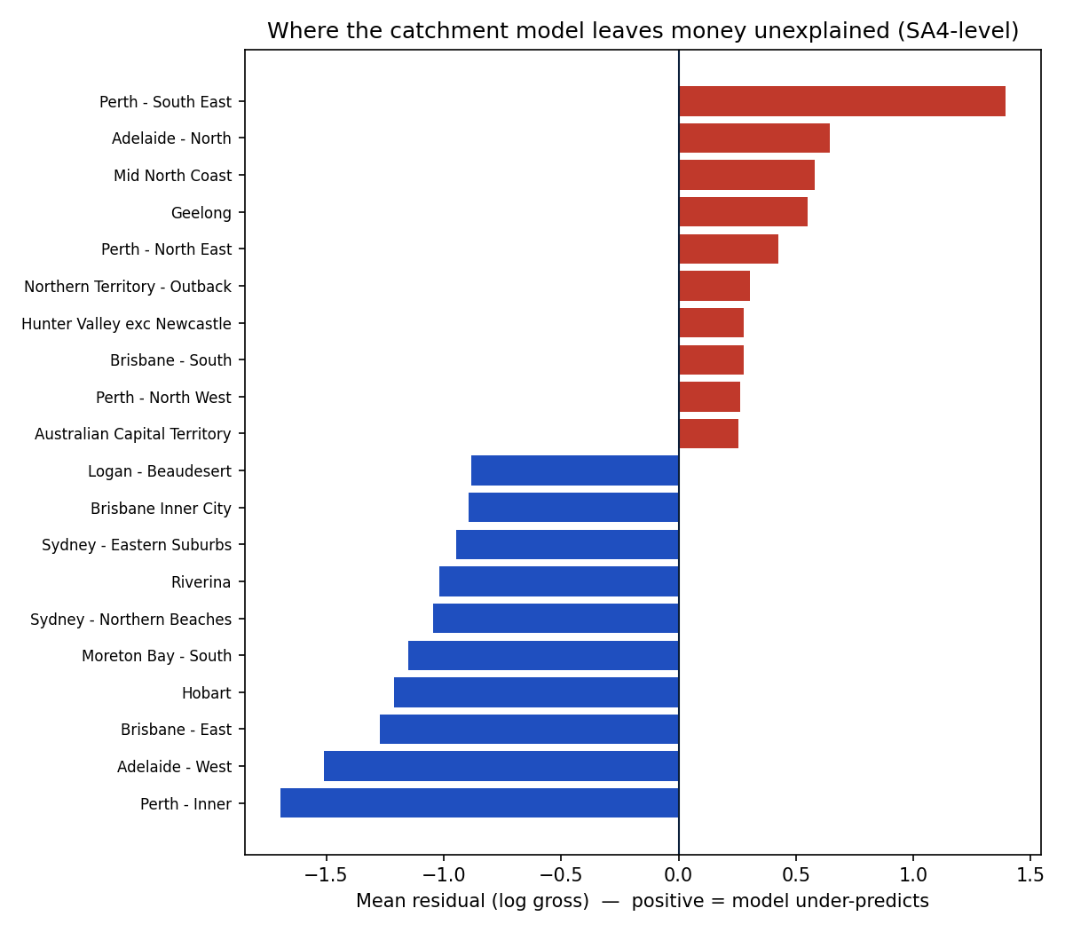
Where the model still leaves money unexplained
SA4-level mean residuals after M3. Positive bars = the catchment model under-predicts demand there, so something beyond demographics is driving it (cinema quality, marketing, community events). Negative = over-prediction.
Caveats
- SA4 polygons are coarse: Sydney's Indian-Australian heartland sits inside a few suburbs (Parramatta, Blacktown) but SA4 spreads that signal across a much larger area. An SA2-level rerun would sharpen the estimate.
- 143 of 198 unique cinemas geocoded. Mostly regional cinemas were excluded; the panel is representative of metropolitan demand.
- Coefficients are conditional associations, not RCT-style causal effects. The fixed effects control for film and week-level shocks, but unmeasured confounders (advertising spend, suburb-level cinema quality) remain.